3 Adaptive coding

The algorithms implemented in the short lab require a probability distribution of all symbols in the whole file to be first calculated and used by both the encoding and decoding process. However, this step may be impractical for three reasons. First, the probability distribution of the whole source may not be known beforehand in applications like live streaming. Second, even if it is known, it will be resource intensive to parse the whole file twice, once to calculate the probability, and the second time to encode the file. Thirdly, the probability distribution needs to be stored and in some cases, transmitted, taking up precious storage and channel resources. Thus, adaptive coding has been devised to obtain the estimated probability distribution and encoding the file at the same time through one parsing, with the mechanism described below.

First, instead of calculating the probability distribution of the source, it assumes a probability distribution to start with. In our implementation, the probability distribution was initiated with a uniform distribution of frequency 1 for 128 ASCII symbols, giving the probability \(1/128\) for each symbol. Next, the first symbol will be encoded using the initial probability model. In the third step, the probability model will be updated by increasing the frequency of observed symbol by 1 and recalculated each symbol’s probability. The second and third step will continue until it reaches the end of file. The implementation is in adaptive_arithm.py

3.1 Laplace smoothing and Laplacian estimator \(\delta\)

A Laplacian estimator, \(\delta\), was used to smooth the calculation of categorical data (i.e. probabilities of discrete sources). Instead of calculating the probability of the symbol as it has been observed, the model assumes that the encoder has observed every symbol in the alphabet \(\delta\) times. Thus, the updated probability of observing symbol \(x\) after observing \(n\) symbols in total and \(n_x\) \(x\) symbols is \(\hat{p_x}\) where \[ \hat{p_x} = \frac{n_x+\delta}{n+k\delta} \] To observe the effect of \(\delta\) on \(\hat{p_x}\), we simulated observing only one symbol in 100 observations. In this simulation, \(p(x) = 1\) and \(k = 128\) and the result is in the figure blow. Figure 3.1 a shows that a small \(\delta\) can converge to \(p(x) = 1\) faster. The larger the \(\delta\), the more influence the initial estimation will have on the probability estimation of the source, and the less variable the probability estimation is. This observation does not mean that a smaller \(\delta\) is necessarily better, because a delta that is too small may “overfit” on the data that it has observed. Even if the prior probability distribution is in fact the source probability distribution, it may converge slower in this case. In the extreme case, \(\delta =0\) will perform badly for the first symbols when the prior probability distribution is not the source probability distribution. Figure 3.1 b shows that the convergence will also occur faster to the true probability when the alphabet size is smaller.

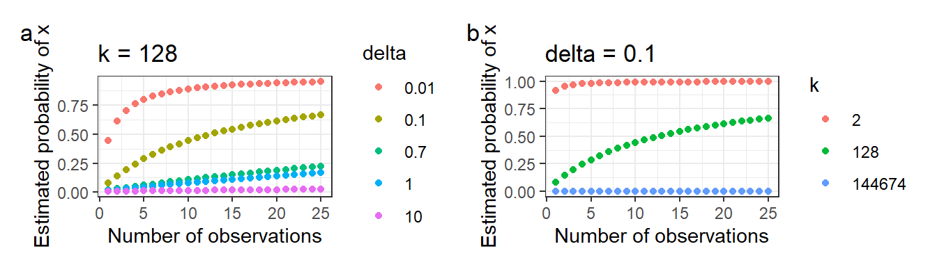
Figure 3.1: Change of estimated probabilities of x (\(\hat{p_x}\)) with number of observations (\(n\)) at different (a) Laplacian estimator, \(\delta\), and (b) alphabet size, k, when \(p(x) = 1\)

3.2 Effect of meausrement length, \(n\), and \(\delta\) on adaptive compression entropy

Comparing the convergence rate to the probability, as done in the last section, is not enough for a comprehensive evaluation of the Laplacian estimator’s effect on compression. Thus, we further evaluated the rate that average code length converges to entropy, as we would expect to occur in a practical static encoder.

The performance of an adaptive code can be estimated by assuming the length of the code word is \(L = -\log\hat{p}\) where estimated probability is \(\hat{p} = -\prod_{i}\hat{p_{x_i}}\) for a string of data \(x_1, x_2, ... ,x_n\). Manipulating using logarithmic properties, the length of the code word can thus be calculated from the probability of each symbol in the string of data as \(L = -\sum_{i=1}^n\log_2\hat{p_{x_i}}\)

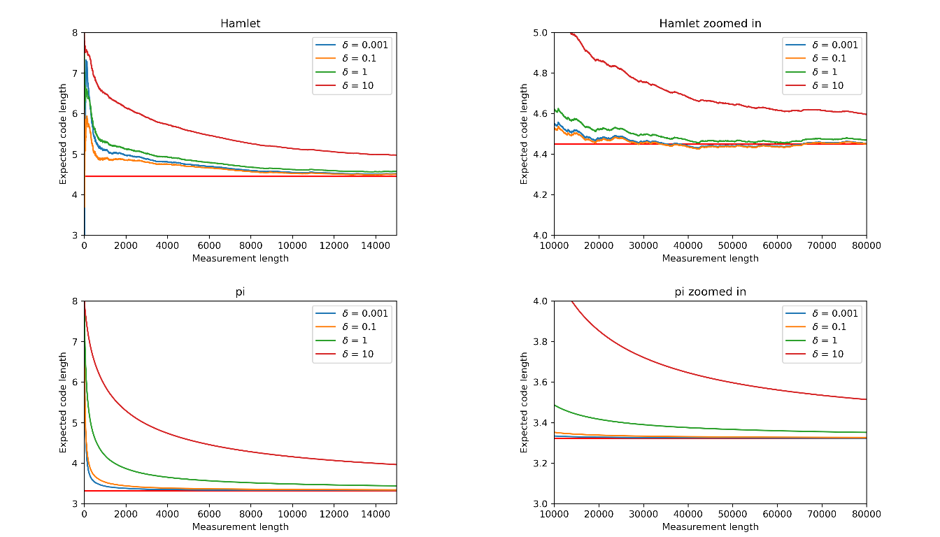
Figure 3.2: Expected code length decreases with increasing measurement length at rate dependant on \(\delta\). Red horizontal line indicates entropy

Shown in the Figure 3.2 , except for the fluctuation at the first few symbols, the average code length decreases with increasing measurement length at different rates depending on \(\delta\) for both Hamlet and pi. The expected code length for both Hamlet and pi achieved source entropy at around 20000 to 30000 measurement length for \(\delta = 0.1\) and \(0.01\). Distinctively, the convergence is slower in pi than in Hamlet when \(\delta = 1\). When \(\delta = 10\), the expected code length did not achieve source entropy in both files. A further comparison of converging rate shows that the decreasing rate is fastest at \(\delta=0.1\) in Hamlet and at \(\delta=0.001\) in pi. Thus, all resulting performance tend to the entropy but at a rate dependent on \(\delta\). This shows the \(\delta\) is most important in deciding the code lengths of the first few symbols of the source stream.

This experiment first demonstrates that an optimal \(\delta\) exists. In Hamlet, decreasing \(\delta\)f first decreases average code length, but further decrease of \(\delta\) at a range between 0.1 and 0.001 result in an increase in average code length. Secondly, this experiment shows that the optimal \(\delta\) can be different for each file source. The optimal \(\delta\) for Hamlet is larger than the optimal \(\delta\) for pi, which could be due to smaller true alphabet size in pi. The optimal \(\delta\) was calculated to be around 0.03 for Hamlet. Other estimators such as Dirichlet and Jelinek-mercer smoothing could also be explored [5].

3.3 Comparison between static and adaptive coding

3.3.1 Compression rate

Static coding has the advantage of knowing the source probability distribution beforehand. Thus, when the prior estimation of the probability distribution is distinct from the source probability distribution, it may be advantageous to use a static coding algorithm, especially when the software is specialised for a specific use case.

For small files, a static encoder may be advantageous before the adaptive encoder converges to source entropy. However, for large files, it is possible that the stationary assumption no longer holds. For example, a text file compiling modern English poems may have a best fitted probability distribution for each writer, but the average probability distribution will be underfitting for most poems. An adaptive coder will be advantageous in this case.

In addition, it will also depends on the type of files. When the alphabet size is small, the probability distribution size will be small, so static coding can be more efficient in terms of storage and transmission. Meanwhile, as we seen in the second Figure above, the convergence rate may also be faster for adaptive coding. Thus, whether adaptive or static coding will be more efficient will further depends on a number of factors including the choice of \(\delta\) and initial distribution. This is further discussed in 5.0.3.

3.3.2 Computation

Both static and adaptive coding have their computationally expensive parts. The static coding requires parsing through the file twice and calculate a probability table by first loading the whole file in to memory, which is unfeasible for large files. Conversely, while adaptive coding can calculate the probability on the fly, for the case of Huffman coding, it is CPU-intensive and slow to re-compute the tree every time. This is further discussed in 5.0.1.

3.3.2.1 Improvement on adaptive Huffman coding

A less computationally expensive adaptive Huffman coding can be based on the Sibling Property, which states that except the root, each node in the tree has a sibling and the non-increasing weight with each node adjacent to its sibling can be used to list the nodes [6]. This allows minimum modification of the trees and therefore practical application. Two examples of adaptive Huffman coding algorithms include the FGK algorithm and the Vitter algorithm [7].