2 Contextual coding
The initial implementation of all coding schemes encoded without context and assumed that each symbol is identically and independently distributed (i.i.d). Practically, for each symbol it encounters, it only considers the probability of that symbol alone. However, in natural language such as English, observing one symbol will often reduce uncertainty as to what the next symbol may be. As a highly cited example in English, the probability of the next letter being “u” is almost 1 when observing “q” as the first letter [2]. Based on this idea, contextual coding builds its probability table with groups of symbol instead of only one symbol.
A helpful statistical model is the notion of the discrete stochastic process, which models the source stream (e.g. Hamlet text) as a sequence of random variables with a joint probability distribution. In particular, we assume that the process of our source stream is stationary i.e. the joint probability of any block of sequence does not change with time as encoder parses through the source. This assumption is highly debatable as it concerns whether the probabilities of any natural languages’ symbols converge after processing “enough” text. Apart from 7, this report will steer clear of the linguistic or philosophical debate and instead focus on the useful properties of this assumption may bring to data compression.
The whole encoding process can be modeled based on a three-state process as the following: from the initial state of discrete stationary source (text), a parser is used to group consecutive n symbols as a block. The joint probability of this block will be used to calculate the code word in a similar process to single-symbol encoding implemented in the short lab. As English symbols are likely to be dependent on previous symbols, the average entropy calculated from the joint probability of \(n\) symbols, \(H_n = \frac{1}{n} H(X_1, ... X_n)\), is expected to be lower than consider each symbol’s probability alone. The entropy rate of a discrete stationary source is defined as \(H_n\) when \(n\) approaches infinity, \(H(X) = \lim_{n\rightarrow\infty}\frac{1}{n} H(X_1, ... X_n)\)
A different perspective of the entropy of a stationary stochastic process can be built on the initial notion that the probability of the next symbol, \(X_n\), is conditional on the symbols proceeding it, which can be defined as \(H^*_n = H(X_n|X_1...X_{n-1})\). It can be proven that both notion are equivalent as \(n\) approaches infinity and both are non-increasing as \(n\) increases. The proofs can be found in the Appendix. \[ H_{\infty}(X) = \lim_{n \rightarrow\infty}H_n =\lim_{n \rightarrow\infty}H^*_n \] if the limit exists (which may not always be the case).
The concept of entropy rate allows us to derive the following relationship with the expected code length of a discrete stationary process, with the proof in the Appendix: \[ H_{\infty}(X) \leq E[L_k]/n < H_{\infty}(X) + \frac{1+\epsilon}{n} \] Viewed together, the two theorems are informative of the achievable code length of a discrete stationary process. It also shows that one can achieve the expected code length by either through block coding or coding based on coditional probability. It further demonstrates that having more \(n\) in the block can only decrease the source entropy rate or make it constant. This implies we should always aim to have a larger block, but the practical repercussions of doing so is discussed in 2.2 and 4.1.
2.1 Implementation of contextual coding
This report will focus on a simple but instructive case where the probability of the next observed symbol only depends on current symbol and not any previous symbols. The whole source stream can be modelled as a Markov process. Assuming the Markov process is aperiodic, irreducible and time-invariant, we can always achieve its steady state distribution [3]. The transition matrix can be modeled as the following:
\[P(\text{next state} | \text{current state}) = \begin{bmatrix} p_{a,a} & \dots & p_{a,z} \\ p_{b,a} & \dots & p_{b,z} \\ \vdots & \ddots & \vdots \\ p_{z,a} & \dots & p_{z,z} \end{bmatrix} \]
When the encoder iterates through the source stream, it will subset the transition matrix according to the current symbol to generate a conditional probability dictionary. This conditional probability dictionary will then be used to generate the code word for the next symbol. An implemntation of the contextual encoder can be found in contextual_arithm.py file.
2.2 Large n in practical applications
2.2.1 Techniques for implementation
One technique to allow \(n\) to be made very large is to enlarge the alphabet. For example, previously we considered alphabet size of 26 from a-z. By increasing the alphabet size to \(26^2\). we can calculate the transition probability from a two-symbol current state to a two-symbol next state, effectively coding four symbols in a block. Another technique is to expand this 2-dimenional matrix into an n-dimensional array filled with probability of the next symbol depending on the previous \(n-1\) symbol.
By Theorem 1 and 2, a large \(n\) will help to achieve a better (at least non-worse) compression rate assuming that the source is not i.i.d. A larger \(n\) could be particularly useful when compressing images due to stretches of repeated symbols. For example, gzip can compress 258 bytes in the deflate format, thereby achieving a maximum compression of 1032:1 [4].
However, as \(n\) increases, the array size and complexity scales exponentially. This adds to the computational power and memory required to compute and store the array. Besides, as the message can only be encoded after the complete block has been received, a large \(n\) also means a greater delay in the system, in addition to the possible higher computational time. Furthermore, the number of possible messages and codeword increases particularly in the case of variable length coding (e.g. Huffman) and this may not be economical for small text files.
2.3 Inaccuracy of entropy rate calculation for large block size and finite source
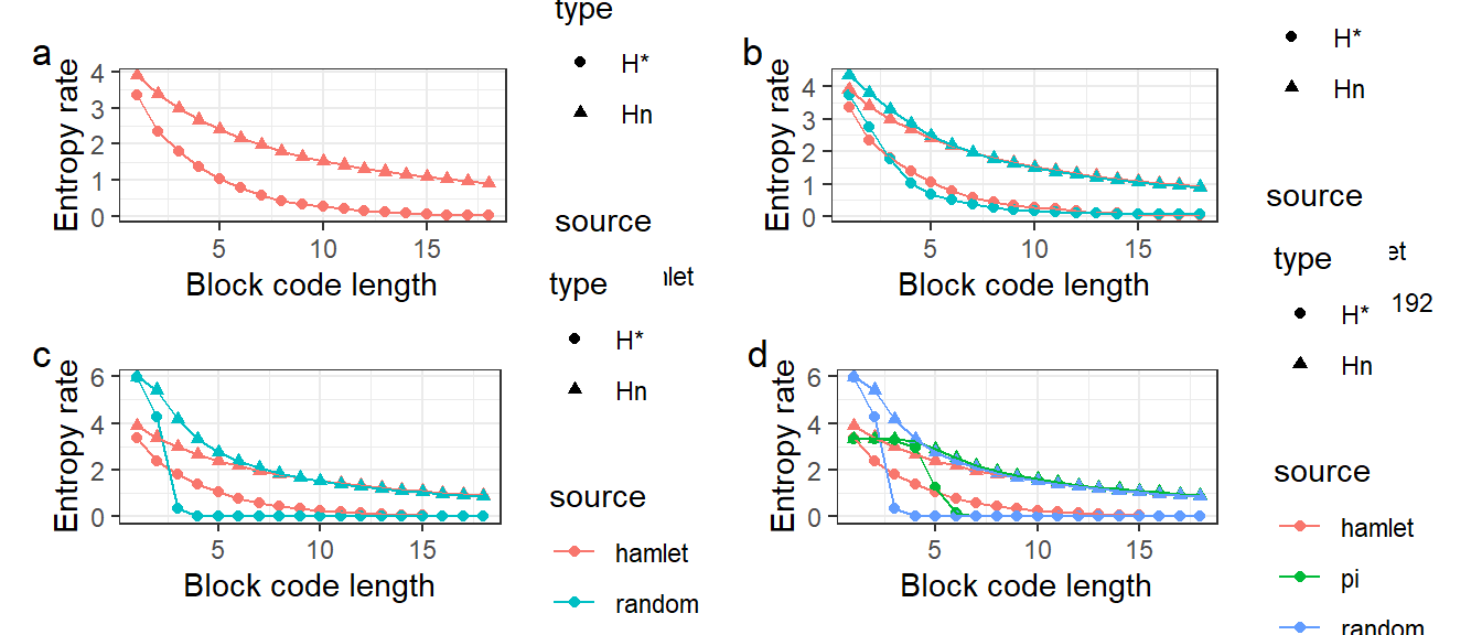
Figure 2.1: Entropy rate estimation of Hamlet, pi and random string at different block lengths. H* refers to conditional entrpy rate \(H^*_n\) and Hn refers to block length entropy rate \(H_n\)
The concept of entropy rate is further explored by measuring the entropy of consecutive symbols of size 2 up to 30. Each file has been truncated to the length of the shortest file, Hamlet. In Figure 1a, the entropy rate measured by block length or conditinal probability decreases. Block length entropy rate \(H_n\) decreases slower than conditional entropy rate \(H^8_n\). The fact that both measurements of entropy rate decreases to zero raises the alarm of the accuracy of the calculation and can be interpreted as the following.
While the first 2 calculations of \(H_n\) and \(H^*_n\) may be approximated to real value, the calculation beyond this point becomes inaccurate. The calculation of entropy rate requires a stochastic process that whose probability of each symbol converges. In this experiment, we have a finite source with a known frequency. The entropy calculation becomes inaccurate for large \(n\), because as the size of the block increases, it becomes relatively significant as compared to the whole source string length. Each block becomes rarer and the probabilities are no longer accurate for calculating entropy. As a result, the source string can no longer be seen as an infinite stochastic process and the entropy rate stops to be a valid property to be calculated. Take an extreme case where the number of consecutive symbols grouped together equals to the length of the source string: the encoder only needs to encode a single binary, 0, to indicate to the decoder to decompress and recover the source file. However, this has no real-world applications since all it does is to decompress one and only one single file that has been agreed upon and stored in the decoder.
Thus, we will focusing on the entropy rate when \(n \le 2\) where calculation can be considered reasonable, Figure 1b shows world192, an encyclopedia, has a larger entropy rate than Hamlet, possibly due to a greater diversity of words. Figure 1c and 1d shows that both pi and random string have higher entropy rate than Hamlet. It should be noted that pi’s entropy rate does not change when \(n le 2\), indicating that the conditional probability on current and previous symbols does not reduce the uncertainty of the next symbol. This fits our intution of \(\pi\) being an irrational and nearly random number. random entropy does decrease, which could reflect either inaccurate calculation or underlying pattern in the random string, possibly due to the pseudorandom number generator. Figure 1c and 1d shows that the entropy rate beyond 3 of a random string (pi and random) can decrease below English text, which is unrealistic and further stresses the point of inaccurate calculation.